"The app is slow" is not a query problem until you have shown it is one. This note follows the order I would actually work in: find which query, read what the database did with it, decide whether the fix is the query, the index, the statistics, or something that is not the query at all.

The single most useful habit: measure before changing anything, and change one thing at a time. Most bad performance work is a pile of speculative indexes nobody can remove because nobody knows which one mattered.

Triage order

1. Which query? pg_stat_statements, ranked by total time — not by mean.
2. What does the planner do with it? EXPLAIN (ANALYZE, BUFFERS).
3. Does the plan match reality? Compare estimated rows to actual rows.
4. If the plan is fine, is the query even the problem? Locks, bloat, pool exhaustion, N+1 from the ORM.

Finding the slow query

CREATE EXTENSION IF NOT EXISTS pg_stat_statements;
 
SELECT
  calls,
  round(total_exec_time::numeric, 1) AS total_ms,
  round(mean_exec_time::numeric, 2)  AS mean_ms,
  rows,
  query
FROM pg_stat_statements
ORDER BY total_exec_time DESC
LIMIT 20;

Order by total time, not mean. A 2 ms query called 400,000 times per minute costs more than a 4-second report that runs hourly, and only one of them is worth your afternoon.

Two companions:

-- log anything slower than 500ms
ALTER SYSTEM SET log_min_duration_statement = '500ms';
 
-- and log its plan automatically
ALTER SYSTEM SET auto_explain.log_min_duration = '500ms';
ALTER SYSTEM SET auto_explain.log_analyze = on;

auto_explain is the one that saves you, because it captures the plan as it ran in production, with production statistics and production parameter values. Re-running the query by hand later often produces a different plan.

Reading a plan

EXPLAIN (ANALYZE, BUFFERS, FORMAT TEXT)
SELECT o.id, c.name
FROM orders o
JOIN customers c ON c.id = o.customer_id
WHERE o.status = 'pending';

EXPLAIN alone shows the plan the planner would choose, with estimates. ANALYZE actually runs it and adds measured values. BUFFERS adds how many pages were read from cache versus disk.

How to read the tree

• The deepest, most-indented node runs first; rows flow upward to its parent.
• Sibling nodes under a join are the two inputs — the first is the outer side.
• Each line's cost and time are cumulative, including its children. To get a node's own cost, subtract its children.
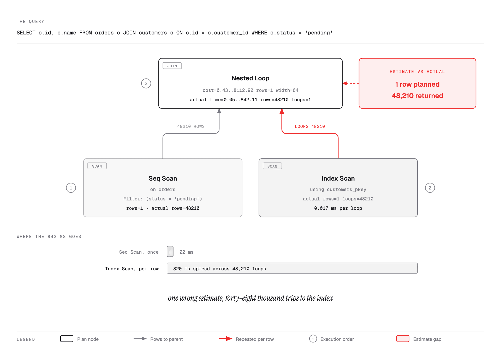
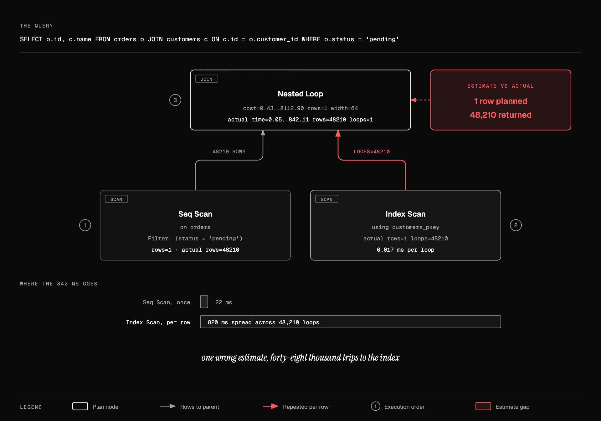
• loops=N means the node ran N times. The reported actual time is per loop. Total time for that node is actual time × loops, and forgetting this multiplication is the most common misreading of a plan.

The numbers

Nested Loop  (cost=0.43..8112.90 rows=1 width=64)
             (actual time=0.05..842.11 rows=48210 loops=1)
  ->  Seq Scan on orders  (cost=0.00..4102.00 rows=1 width=32)
                          (actual time=0.01..38.42 rows=48210 loops=1)
        Filter: (status = 'pending')
        Rows Removed by Filter: 951790
  ->  Index Scan using customers_pkey on customers
                          (actual time=0.01..0.01 rows=1 loops=48210)

rows=1 estimated, rows=48210 actual. That single mistake produced the whole problem: the planner thought a nested loop would probe the inner side once, so it chose one. It ran 48,210 times instead. The join is not slow because nested loops are bad — it is slow because the plan was built on a number that was wrong by five orders of magnitude.

A large estimate/actual gap is the first thing to look for in any plan. Fixing the estimate usually fixes the plan without you touching the query.

Rows Removed by Filter: 951790 is the other line worth reading: nearly a million rows were read and thrown away, which says the filter belongs in an index.

With BUFFERS you also get shared hit= (from cache) and shared read= (from disk). A high read count on a query you expect to be hot means the working set does not fit in shared_buffers.

Why the estimate was wrong

• Stale statistics. Run ANALYZE orders;. Autovacuum normally handles this, but a bulk load can outrun it.
• Insufficient sampling. For a large table with skewed values, raise the target and re-analyze:

  ALTER TABLE orders ALTER COLUMN status SET STATISTICS 1000;
  ANALYZE orders;

• Correlated columns. The planner assumes independence. If city and postcode are correlated, it multiplies two selectivities and gets a number far too small. Tell it:

  CREATE STATISTICS orders_city_post (dependencies, ndistinct)
    ON city, postcode FROM orders;
  ANALYZE orders;

Scan types

A Seq Scan is not a bug. On a 500-row table it is faster than any index. On a query returning 40% of a large table it is also faster, because random heap fetches cost more than sequential reads. Worry when a Seq Scan feeds a tiny result set.

Index Only Scan needs one extra thing people miss: the visibility map must say the pages are all-visible, which is maintained by vacuum. A table with heavy churn and lazy autovacuum will show Heap Fetches: climbing on what should be an index-only scan, and the fix is vacuum, not a new index.

Join strategies

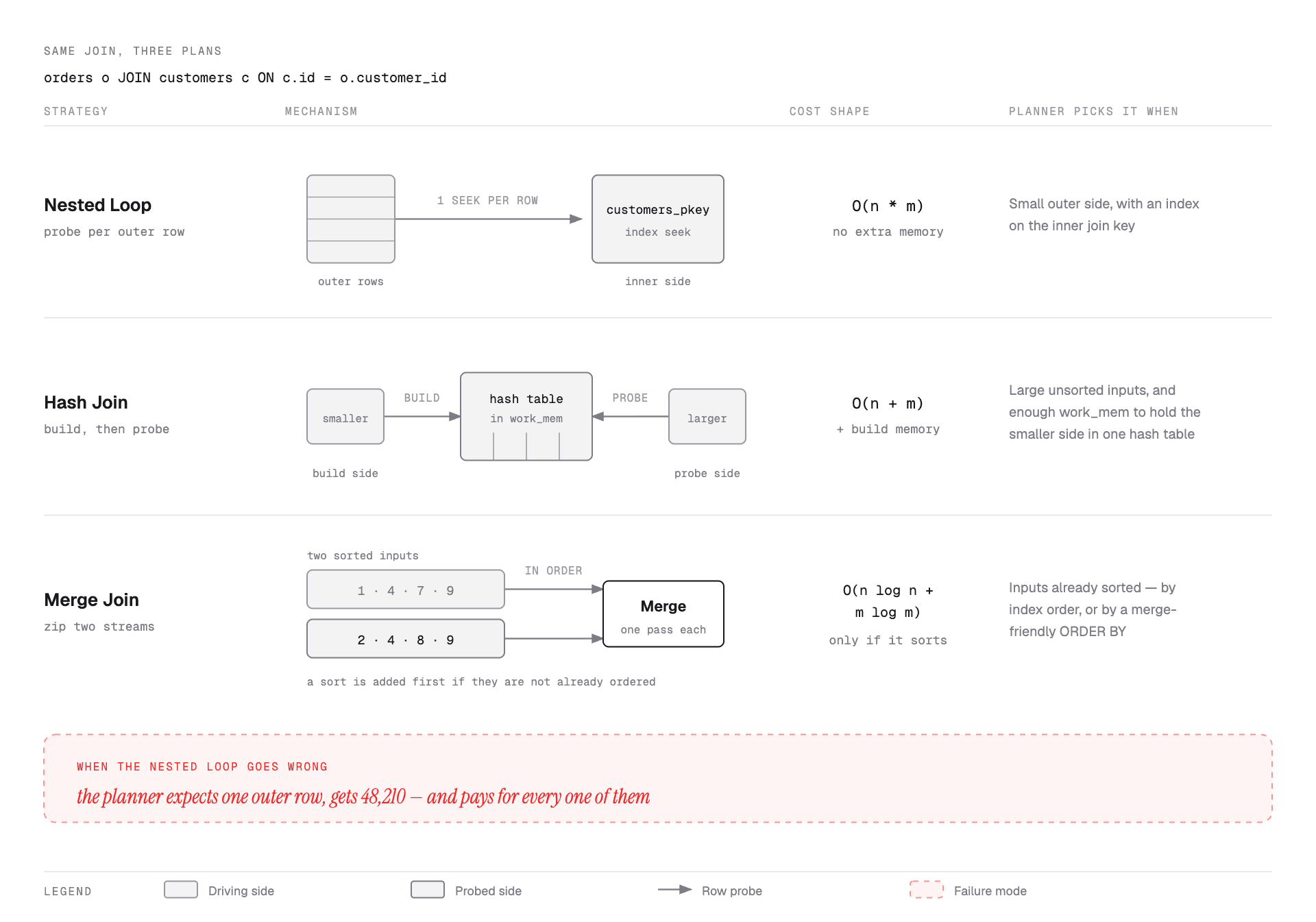
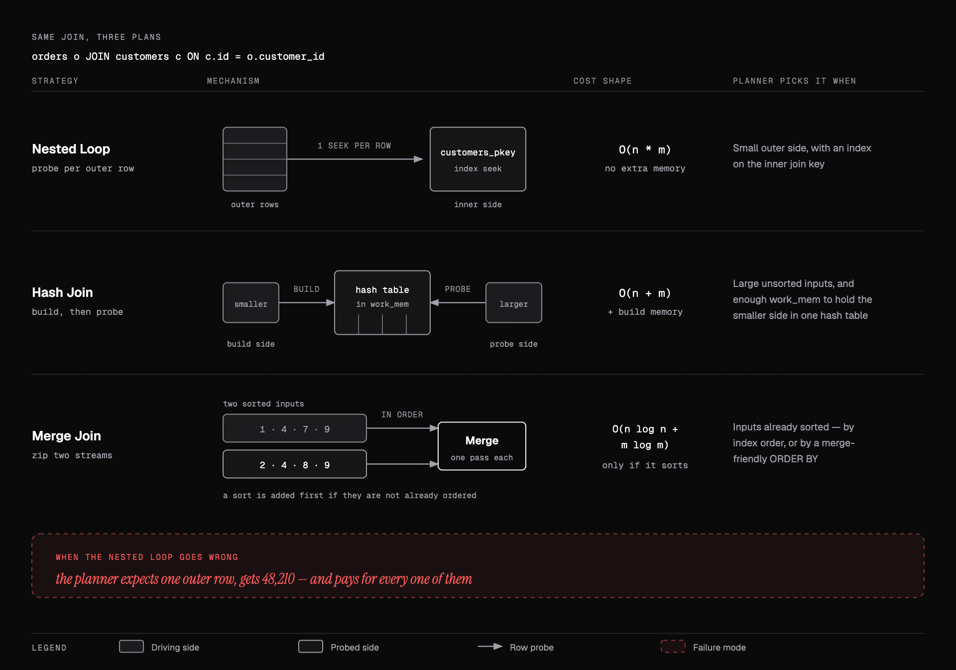
Nested Loop. For each row of the outer input, probe the inner. Cost is roughly outer × inner_lookup. Excellent when the outer side is small and the inner has an index on the join key. Catastrophic when the outer side turns out to be 48,210 rows instead of 1.

Hash Join. Build a hash table from the smaller input, then stream the larger one through it. Roughly O(n + m), but the hash table needs memory: if it exceeds work_mem it spills to disk in batches and gets much slower. Requires an equality condition.

Merge Join. Advance through two sorted inputs together. Great when both are already sorted — typically from index order. If a sort is required first, that sort costs O(n log n) and often loses to a hash join.

You rarely choose these directly. You influence them by fixing statistics, by adding an index that makes one side cheap, or by raising work_mem for a specific session. Disabling a node type with SET enable_nestloop = off is a diagnostic, to confirm the alternative would be faster. Shipping it is not a fix.

Indexes

Composite order and the leftmost prefix

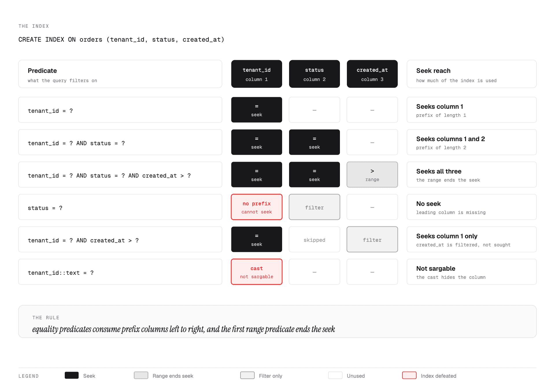
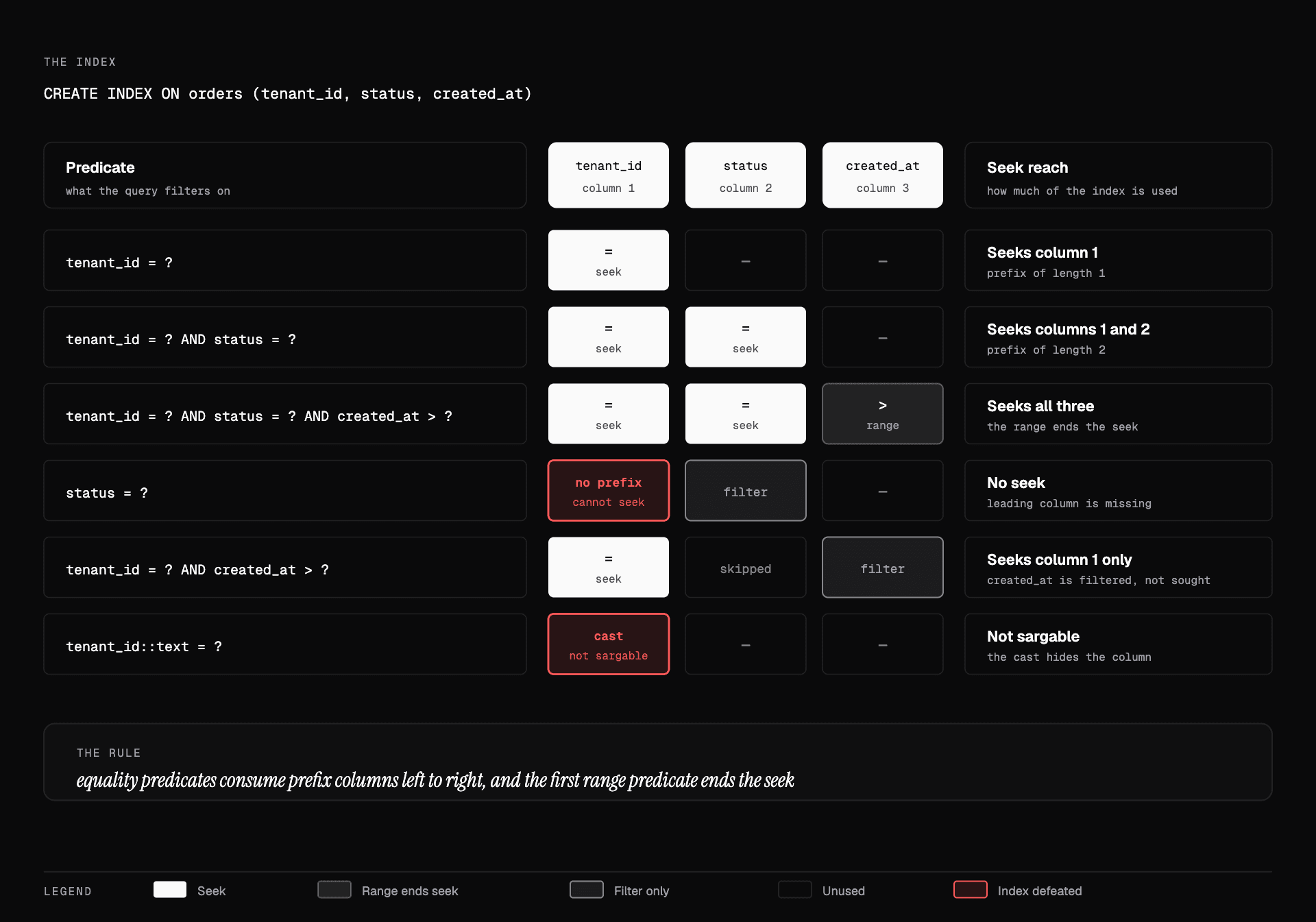
Given:

CREATE INDEX orders_tenant_status_created
  ON orders (tenant_id, status, created_at);

A B-tree is sorted by the tuple, so it can only seek on a leftmost prefix:

The rule: equality predicates consume prefix columns left to right; the first range predicate ends the seek. Everything after a range is a filter, not a seek. So put equality columns first, the range column last, and the column you ORDER BY in a position where the index can also supply the ordering.

Sargability

A predicate is sargable if the database can use it to seek. These are not:

WHERE lower(email) = 'a@b.com'         -- function on the column
WHERE created_at::date = '2026-01-02'  -- cast on the column
WHERE tenant_id::text = '42'           -- implicit type mismatch
WHERE description LIKE '%urgent%'      -- leading wildcard
WHERE amount * 2 > 100                 -- arithmetic on the column

Each wraps the indexed column in something the index does not know about. The fixes:

CREATE INDEX ON users (lower(email));                        -- expression index
WHERE created_at >= '2026-01-02' AND created_at < '2026-01-03';  -- range, not cast
WHERE tenant_id = 42;                                        -- match the type
CREATE INDEX ON docs USING gin (to_tsvector('english', body));   -- real full-text
WHERE amount > 50;                                           -- move the maths

Keep the column bare on the left-hand side. That is the whole heuristic.

Partial, covering, expression

-- partial: index only the rows you query
CREATE INDEX ON jobs (created_at) WHERE status = 'pending';
 
-- covering: extra columns stored in the index for index-only scans
CREATE INDEX ON orders (tenant_id, created_at) INCLUDE (total_cents);

A partial index on a hot subset can be a fraction of the size of the full index, which means more of it stays in cache.

What indexes cost

Every index is written on every INSERT, UPDATE (of an indexed column) and DELETE. Ten indexes turn one row write into eleven. They also consume cache that the table's own pages wanted.

Find the ones nobody uses:

SELECT relname, indexrelname, idx_scan
FROM pg_stat_user_indexes
WHERE idx_scan = 0
ORDER BY pg_relation_size(indexrelid) DESC;

Check uptime before trusting that — an index used only by a quarterly report will show zero scans on a database restarted last week.

When the query was never the problem

This section is what separates someone who has run a production database from someone who has read about one.

Lock waits

The query is not slow; it is waiting.

SELECT pid, wait_event_type, wait_event, state,
       now() - query_start AS duration, query
FROM pg_stat_activity
WHERE state != 'idle'
ORDER BY duration DESC;

wait_event_type = 'Lock' means blocked. pg_blocking_pids(pid) names the blocker. The classic shape: one long transaction left idle in transaction holding a lock, and fifty queries queued behind it. Set idle_in_transaction_session_timeout so that cannot persist.

The migration version of this is in the schema changes note: one ALTER TABLE waiting for a lock blocks every query that arrives after it.

Bloat and vacuum

PostgreSQL's MVCC leaves dead tuples behind on UPDATE and DELETE. Autovacuum reclaims them. When it falls behind, tables and indexes grow with dead space, and every scan reads more pages for the same rows.

SELECT relname, n_live_tup, n_dead_tup, last_autovacuum
FROM pg_stat_user_tables
ORDER BY n_dead_tup DESC LIMIT 10;

A long-running transaction — including an idle one, and including a replica with hot_standby_feedback on — holds back the horizon and prevents vacuum from cleaning anything newer, anywhere in the database. A reporting query left open for six hours can bloat tables it never touched.

Connection pool exhaustion

Latency graphs look identical to slow queries, but the queries are fine — requests are waiting for a connection. Each PostgreSQL connection is a process with real memory cost; a few hundred is a lot. If your app opens 500 connections, you need PgBouncer in transaction mode in front, and an app pool sized to what the database can actually serve concurrently.

Symptom to recognise: p99 latency rises sharply while pg_stat_statements mean times stay flat. The time is being spent before the query starts.

Sorts and hashes spilling to disk

Sort Method: external merge  Disk: 24560kB

That means work_mem was too small and the sort went to disk. work_mem is per sort node, per connection — a query with three sorts across 100 connections can allocate 300× your setting. Raise it for the session that needs it rather than globally:

SET LOCAL work_mem = '64MB';

N+1 from the ORM

Still the most common cause of a slow page, and it never shows up as a slow query — it shows up as 201 fast ones.

const orders = await db.order.findMany({ where: { status: "pending" } });
for (const order of orders) {
  order.customer = await db.customer.findUnique({ where: { id: order.customerId } });
}

Each individual query is 0.4 ms and perfectly indexed. The page takes 900 ms. EXPLAIN on any one of them tells you nothing.

Find it by counting queries per request, not by timing them. Fix it by loading in one round trip — a join, or a second query with WHERE id = ANY($1) and an in-memory map.

Deep pagination

LIMIT 20 OFFSET 200000 reads 200,020 rows and discards 200,000. Covered in full in the API note; worth recognising here because in a plan it appears as a large Seq Scan or Index Scan feeding a Limit node whose actual row count is tiny.

Partitioning

For tables large enough that maintenance, not lookup, is the problem. Range partitioning by time is the common case:

CREATE TABLE events (
  id bigserial,
  occurred_at timestamptz NOT NULL,
  payload jsonb
) PARTITION BY RANGE (occurred_at);
 
CREATE TABLE events_2026_01 PARTITION OF events
  FOR VALUES FROM ('2026-01-01') TO ('2026-02-01');

The wins are partition pruning (queries with a date predicate touch one partition) and DROP TABLE events_2025_01 replacing a DELETE of 50 million rows — instant, and no bloat.

The catch: every query without the partition key scans every partition, and unique constraints must include the partition key. Partitioning a table whose queries do not filter on the partition key makes things worse.

Caching, last

Caching is correct when the data is genuinely reused and staleness is acceptable. It is a mistake when it is the first response to a slow query, because you have kept the slow query and added invalidation as a new source of bugs.

Order of preference: fix the plan, fix the index, fix the query, denormalize a measured read path, then cache.

Practice

Recall checklist

• Rank by total time, not mean, and say why
• What ANALYZE and BUFFERS each add to EXPLAIN
• Which node in a plan runs first, and how cumulative cost works
• What loops=N does to the reported time
• Why the estimate/actual gap is the first thing you look at
• Three reasons an estimate can be wrong, and the fix for each
• Four scan types and when each is correct
• What an index-only scan needs besides the right columns
• Three join strategies, their cost shapes, and when the planner picks each
• State the leftmost-prefix rule, including what a range predicate does to it
• Five non-sargable predicates and their rewrites
• What every extra index costs on write
• How to tell a lock wait from a slow query
• How one idle transaction can bloat tables it never touched
• The signature of connection pool exhaustion in the metrics
• Why work_mem is dangerous to raise globally
• Why N+1 never shows up in a slow query log
• The two real wins from partitioning, and the case where it backfires